Software
Example Usage:
$ ./image -help
Some Basics
Pixel is the basic unit of programmable color in a computer image. Each pixel is a sample of an original image. The intensity of each pixel is a variable. A pixel is typically represented by three or four component intensities such as red, green, and blue, which are typically in the range of 0 – 255, this is also known as the RGB color model.
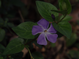
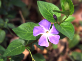
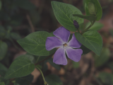
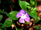
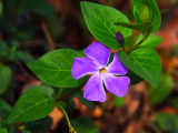
Changing Brightness
To adjust image brightness, we simply scale each RGB component of a pixel by a positive factor α, When α is 0, we get a pure black image, when α is 1 we get the original image back. In other words, if we want to darken the image, we interpolate between the zero RGB intensities (black image) and the current image. Note that linear interpolation is often used to blend two images by interpolating between between corresponding pixel values of the two images as in the following example, where α and (1 - α) are used in a weighted average to obtain the interpolated pixel values:
output_rgb_component = (1 - α) * black_rgb_component + α * input_rgb_component
Since black RGB component is 0, we can simplify the formula:
output_rgb_component = α * input_rgb_componentWe can also obtain the brightened image through extrapolation.
Note: To see full rez image, you'll need to open the image in a new tab
-
0.0

Black Image -
0.5
-
1.0

Input Image -
1.5
-
2.0
Example Usage:
$ ./image -brightness 1.5 <input.bmp >.out.bmp
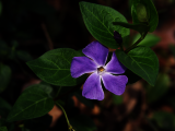
Changing Contrast
Contrast is the difference in luminance that makes an object distinguishable. It can be controlled by interpolating and extrapolating between a constant grey image and the current image just like how we control brightness with a contract factor α. Interpolation reduces contrast and extrapolation boosts the contrast. The grey image is obtained by calculating the average image luminance and assign each grey pixel’s rgb components to the same average image luminance. Note that when a pixel’s rgb components are of the same value, it is on the grayscale. Here is one way to calculate pixel luminance (http://www.itu.int/rec/R-REC-BT.601):
pixel_luminance = (0.299 * R + 0.587 * G + 0.114 * B)
Then apply interpolation on all rgb component for each pixel in the image as follows:
output_rgb_component = (1 - α) * average_pixel_luminance + α * input_rgb_componentA contrast factor of 0 produces a grey image with no contrast, 1 gives the original image, between 0 and 1 loses contrast, greater than 1 increases contrast, and less than 0 inverts the image.
-
-1.0
-
0.0

Grey Image -
0.5
-
1.0

Input Image -
2.0
Example Usage:
$ ./image -contrast 1.5 <input.bmp >.out.bmp
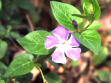
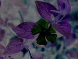
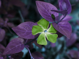
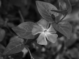
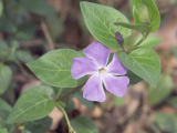
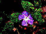
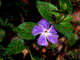
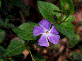
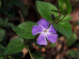
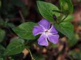
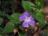
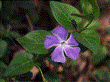
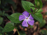
Changing Saturation
Saturation refers to the perceived intensity of a specific color. It is the purity of the color and represents the amount of grey in proportion to the hue. To control the saturation of an image, pixel components must move towards or away from the pixel's luminance value. In other words, we interpolate between the grayscale version of the input image and the input image using the saturation factor α. The grayscale image is obtained by calculating a unique luminance per pixel using the same pixel luminance calculation discussed in the above section. Then apply the same interpolation technique as follows:
output_rgb_component = (1 - α) * current_pixel_luminance + α * input_rgb_componentWhen α is 0, we obtain the grayscale version of the image; when α is 1, we obtain the original input image. So when α is between 0 and 1, it makes the image grayer, reducing the saturation of the colors. For α bigger than 1, we extrapolate increasing saturation. As for negative values, the hues or colors of the input image is inverted, like a photographic negative.
-
-1.0
-
0.0
Greyscale Image -
0.5

-
1.0

Input Image -
2.0
Example Usage:
$ ./image -saturation 1.5 <input.bmp >.out.bmp
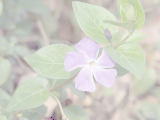
Changing Gamma
Some images are not corrected for the nonlinear relationship between pixel value and displayed intensity for a color monitor. This nonlinear relationship can be described by a function raised to the power of gamma (γ):
displayed_intensity = rgb_component γ
Gamma correction corrects this by applying the inverse of this relationship to pixel values for all pixels in an image. Normally, input RGB component and output RGB component are in the range of 0 – 1; if the input RGB component is in the range of 0 - 255, we divide that component by 255 to normalize it:
normalized_input_rgb_component = input_rgb_component / 255When γ is 1, the output image is unchanged, γ greater than 1 brighten it, and lower values darken it. Note that γ should be positive. If γ is 0, the output is a black image; if γ is smaller than 0, no processing is done and the output is the input image.
normalized_output_rgb_component = normalized_input_rgb_component (1.0 / γ)
output_rgb_component = normalized_output_rgb_component * 255
-
γ = 0.0

-
0.5
-
1.0

Input Image -
2.0
-
8.0
Example Usage:
$ ./image -gamma 2.0 <input.bmp >.out.bmp
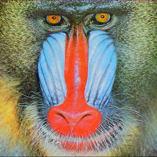
Cropping Images
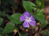
This allows one to crop the image, for instance to focus on a mandrill’s eye or nose as shown in the cropped picture below. The algorithm works by copying pixels at appropriate positions based on the offset x and y from a contiguous 1d array in the original image to a new image with newly specified width and height. We assume that x ranges from 0 to width-1 from left to right and y from 0 to height-1 from top to bottom. w and h are the size of the cropped image.
-
Original Image (512 x 512)
-
Cropped Image: x=0, y=0, w=512, h=512
-
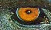
Cropped Image: x=120, y=35, w=100, h=60
-
Cropped Image: x=160, y=80, w=180, h=370
Below shows how we handle some interesting edge cases:
- Case 1: If any of x, y, w, or h are negative, the output is an empty image.
- Case 2: If cropped image dimension exceeds original image bounds, that is if cropping parameter w, h larger than the original image height and width. Then the cropped image will only contain the captured portion of the original image, i.e. cropped_image_max_height = original_image_height - y
- Case 3: If x or y exceeds original image bounds then the output is an empty image
- Case 4: If w or h are 0 then the output is an empty image
-
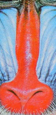
Case 2: x = 150, y = 50, w=15000, h=100
Example Usage:
$ ./image -crop 150 50 100 100 <input.bmp >.out.bmp
Quantization and Dithering
Dithering is used to create the illusion of "color depth" in images with a limited color palette using color quantization and reducing quantization errors. For example, when dithering an image from 8-bit color to 1-bit color, the colors that are available in the 8-bit color palette are approximated by a diffusion of colored pixels from the available 1-bit color palette. We have implemeted various techniques for dithering images with a small number of bits (1-8 bit) that we'll discuss below.
Quantize
Color quantization is a process that reduces the number of distinct colors used in an image. To quantizes the image we use "nbits" per color channel. We first need to define a map between the input, say 8-bit [0 - 255] and the output [0 - (2nbits - 1)]. Note that we only support nbits between 1 and 8 in our implementation. A simple way of doing this is to first convert all values into floating point to lie between 0 and 1 (by dividing the input by 256). Then, select the quantum using
q = floor ( p / 256.0 * b )
where q is the appropriate quantum, p is the original pixel value in the range from 0 to 1, and b is the number of bins or quanta and is calculated using
b = 2nbits
These values must then be mapped back into the 0 - 255 range to obtain the final colorc cf
cf = floor ( 255 * q / (b - 1) )
Note that a fast way for calculate b = 2nbits is to use bit shifting in c++
b = 1 << nbits
The problem with quantization is that it introduces a clear contouring for lower numbers of bits. To prevent this from happening we will need to handle quantization errors better. Dithering is such a process that can distribute errors among pixels to obtain better results. We have implemented two dithering algorithms here: Random Dither and Floyd-Steinberg Dither.
Example Usage:
$ ./image -quantize 2 <input.bmp >.out.bmp
Random Dither
Random Dither was the first attempt to correct the contouring produced by fixed thresholding. Random Dither adds some noise before quantizing. The noise helps to break up the contouring. Perceptually, noise is found to be preferable since human eyes are more tolerant of high-frequency noise than contours or aliasing. In addition to the quantization process above, we add noise in the range from [-.5 ... +.5] when selecting the quantum as shown below.
q = floor ( p / 256.0f * noise )Note that noise can be generated using the random function.
Example Usage:
$ ./image -randomDither 2 <input.bmp >.out.bmp
Floyd-Steinberg Dither
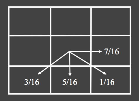
A more advanced dithering algorithm is the Floyd-Steinberg Dither. It achieves dithering using error diffusion, meaning it pushes the residual quantization error of a pixel onto its unprocessed neighboring pixels to be dealt with later. Specifically, the error is split and diffused out with the weights
Right: α = 7/16
Bottom Left: β = 3/16
Bottom: γ = 5/16
Bottom Right: δ = 1/16
Error diffusion reduces net errors which gives better result in comparison to Random Dither.
As shown in the image below (courtesy of Ravi Ramamoorthi), we diffuse the error for each pixel:
 Pseudocode:
alpha = 7.0 / 16.0
beta = 3.0 / 16.0
gamma = 5.0 / 16.0
delta = 1.0 / 16.0
for each y from top to bottom
for each x from left to right
oldpixel = pixels[x][y]
newpixel = quantize(oldpixel) // quantize() returns the quantized pixel
pixels[x][y] = newpixel
quant_error = oldpixel - newpixel
pixels[x + 1][y ] += quant_error * alpha
pixels[x - 1][y + 1] += quant_error * beta
pixels[x ][y + 1] += quant_error * gamma
pixels[x + 1][y + 1] += quant_error * delta
Note that the pseudocode above assumes all pixels always have 4 valid neighboring pixels, which means it does not deal with pixels on the edges of the image. To handle the edge condition, we can renormalize diffusion weights based on number of valid neighboring pixels to prevent darkening of edge pixels. The weights are renormalize in a way such that errors being diffused sum up to be the quantized error. For example, if the current pixel being quantized is on the right edge then there are no pixels to the right of it, so only the bottom pixel and the bottom left pixel are valid (assume the quantized pixel is in the middle of the image so there are pixels below it), therefore we only diffuse errors to these two pixels and the renormalized weights are γ' = 5/8 for bottom pixel and β' = 3/8 for bottom left pixel.
for each y from top to bottom
for each x from left to right
...... do quant_error calculation ......
if (pixels[x+1][y] && pixels[x-1][y+1] && pixels[x][y+1] && pixels[x+1][y+1])
// If all neighboring pixels are valid
alpha = 7.0 / 16.0
beta = 3.0 / 16.0
gamma = 5.0 / 16.0
delta = 1.0 / 16.0
...... do error diffusion on valid pixels ......
else if (pixels[x+1][y] && ! pixels[x-1][y+1] && pixels[x][y+1] && pixels[x+1][y+1])
// If left bottom pixel is invalid, no need for β
alpha = 7.0 / 13.0
gamma = 5.0 / 13.0
delta = 1.0 / 13.0
...... do error diffusion on valid pixels ......
else if (! pixels[x+1][y] && pixels[x-1][y+1] && ! pixels[x][y+1] && pixels[x+1][y+1])
// If right and right bottom pixel are invalid, no need for α and δ
beta = 3.0 / 8.0
gamma = 5.0 / 8.0
...... do error diffusion on valid pixels ......
else if (pixels[x+1][y] && ! pixels[x-1][y+1] && ! pixels[x][y+1] && ! pixels[x+1][y+1)
// If only the right pixel is valid, push all error onto that pixel
pixels[x+1][y] += quant_error
else if (pixels[x][y+1])
// If only the bottom pixel is valid, push all error onto that pixel
pixels[x][y+1] += quant_error
else
// if no neighboring pixels then discard the error and do nothing
Example Usage:
$ ./image -FloydSteinbergDither 2 <input.bmp >.out.bmp
Result Comparison
Original Image
Quantization
-
1
-
2
-
3
-
4

-
5

Random Dither
-
1
-
2
-
3
-
4
-
5
Floyd-Steinberg Dither
-
1
-
2
-
3

-
4
-
5
Discrete Convolution
Discrete convolution is important in helping us implementing interesting effects such as blur, sharen and basic edge detection. The idea is to fill in each pixel for the new image by convoling with pixels in the old image the following way
Inew(a, b) = Σ x=(a - w) to (a + w) Σ y=(b - w) to (b + w) h(x-a, y-b) Iold(x, y)Where Inew is the intensities of the new pixel sampled at position (a,b), w is kernel width, h is the filter and Iold is the intensities of the pixel to be sampled in the old image.
Blur
A Gaussian blur is typically used to reduce image noise and reduce detail. We implemented a Gaussian blur here by convolving the image with a Gaussian filter. In 1D, it is described by the function
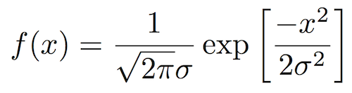 where σ is the kernel width. For 2D filters, we simply obtain f(x,y) = f(x)f(y). We use the above equation to generate a kernel of old width (i.e. 3, 5, 7, 11...), then apply the kernel centered at each pixel calculate a new value using its neighbors. Before doing so, we convert it to a integer based kernel by first dividing it by the smallest value (the furthest from the center of the kernel). Then normalizing it to it doesn't affect the brightness of the picture by dividing the kernel by the sum of its values, then after generating a new value for the main pixel, we multiply it by the normalizing factor to get the right pixel color values. The idea here is that each pixel becomes a weighted sum of the pixels close to it, the closer the pixels are to the center pixel, the more weight they carry.
-
Original Image
-
kernel width = 3
-
5
-
7

-
11
-
Original Image

-
kernel width = 3
-
5
-
7

-
11

Example Usage:
$ ./image -blur 3 <input.bmp >.out.bmp
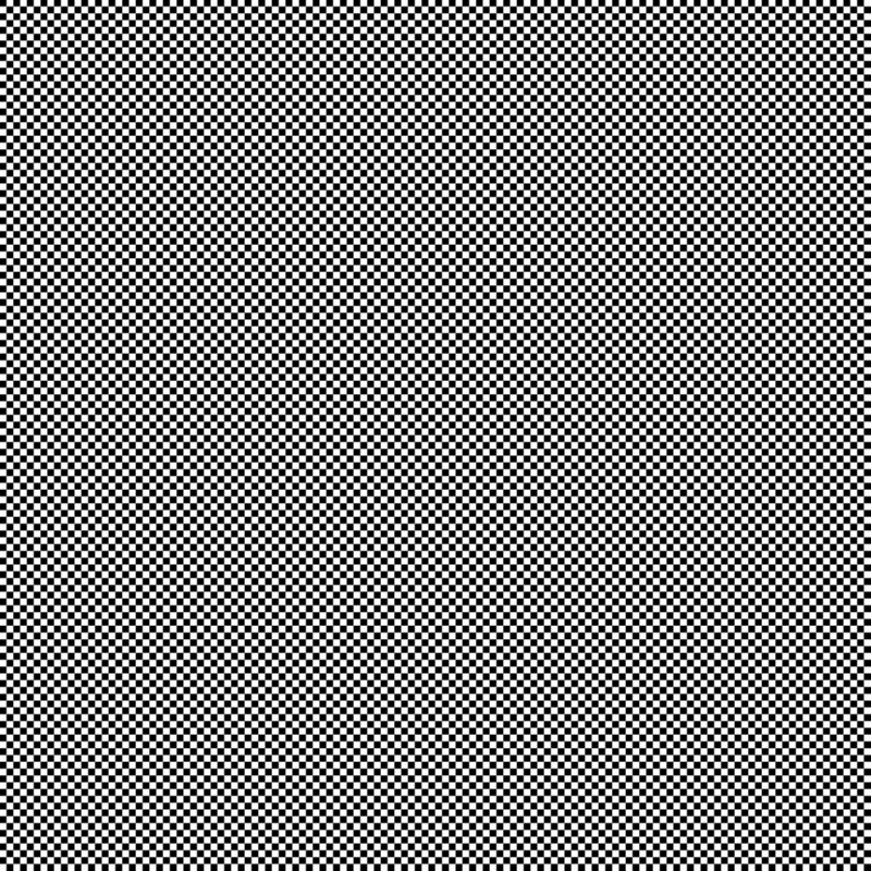
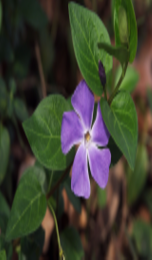
Sharpen
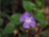
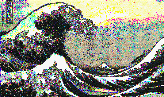
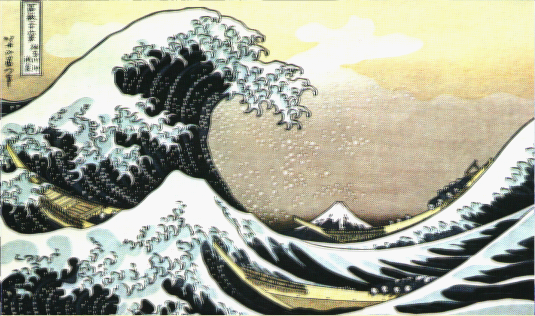
To sharpen an image, we used the same convolution function given and simply passed the filter given in the class, as well as the normalizer. We had unknown issues with pink noises showing up when sharpening some images, as in the example of wave below.
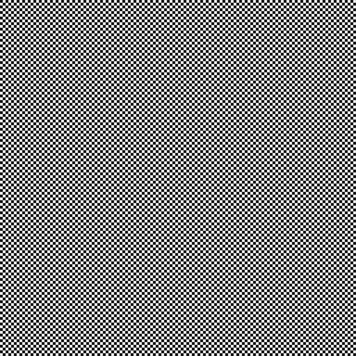
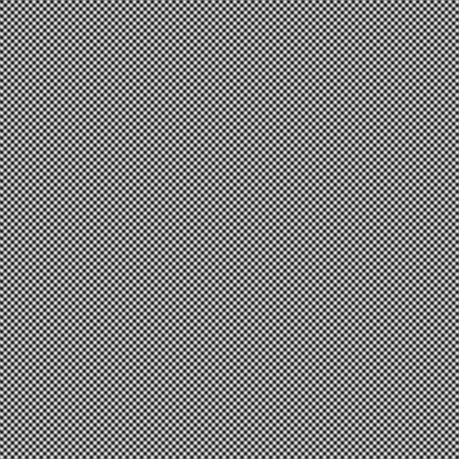
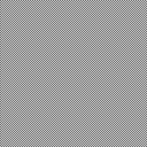
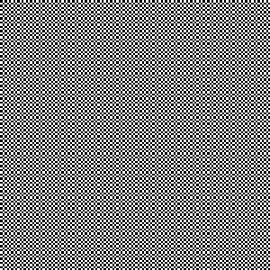
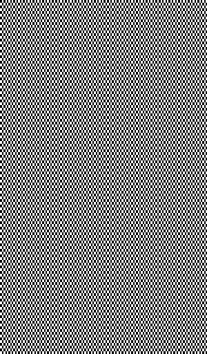
Checkerboard:
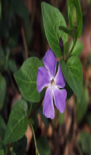
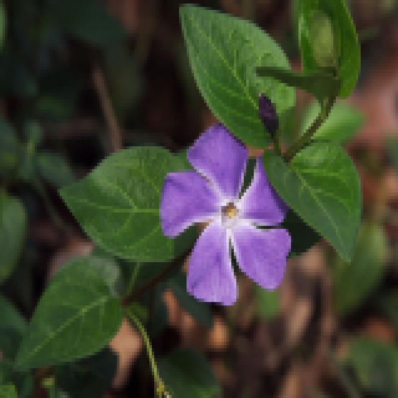
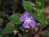
Flower:

Wave looks off, it's got pink noises in it.
Example Usage:
$ ./image -sharpen <input.bmp >.out.bmp
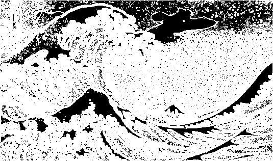
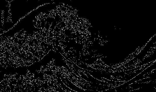
Edge Detection
To do edge detection, we apply the sobel horizontal (and vertical) filters to a grayscale version of the image. The Filters simply ignore the current row (or column), weigh the top row (left column) positive and the the bottom row (right side) negative. That way, you can check the difference in luminance around a certain pixel, if either are high then the image is an edge in the image. Then, based on a passed threshold, you determine whether its color is white (it is an edge/important point) or black (it’s not important).
-
Original Image
-
threshold = 10
-
150

-
200

-
255
Example Usage:
$ ./image -edgeDetect 100 <input.bmp >.out.bmp
Antialiased Scale and Shift
We implemented image scaling and shifting by a real (non-integer) value using three different filters. The first one is nearest neighbor sampling; it is a naive approach that leads to significant aliasing and jaggies. Aliasing is usually caused by under-sampling or poor reconstruction. The second one is a linear filter called hat filter and the third one is a cubic filter called Mitchell reconstruction filter. Both of those filters try to achieve anti-aliasing using convolution.
Nearest Neighbor Sampling
Nearest neighbor or point reconstruction simply samples the nearest pixel in the original image to reconstruct each pixel in the target image. For example, say if you scale an image in y direction by sy and x direction by sx, let's define the operation to be the transformation from (u, v) to (x, y) where (u, v) is the warped location in the source image, or old coordinate and (x, y) is the new coordinate in the transformed image. The pixel at (x, y) in the transformed image is sampled from the (u, v) in the original image, where u = round(x / sx), v = round(y / sy).
Hat Filter
Hat filter is a linear filter that does bilinear interpolation instead of point sampling. It is described by the function
f(x) = 1 - |x|where f(x) is none zero when |x| <= 1. For image processing, we construct the 2D bilinear filter from this 1D linear filter by multipling them together: f(x, y) = f(x)f(y)
Mitchell Reconstruction Cubic Filter
Mitchell Reconstruction Cubic Filter is an extension of cubic interpolation. This is a good finite filter that approximates ideal sync without ringing or infinite width. In contrast to nearest neighbor or linear filter, it produces a smoother image with fewer artifacts. It is described by the function
f(0 <= |x| <= 1) = (7 |x|3 - 12 |x|2 + 16 / 3) / 6For processing 2D images, we use the bicubic filter f(x, y) = f(x)f(y).
f(1 <= |x| <= 2) = (-7/3 |x|3 + 12 |x|2 - 20 |x| + 32 / 3) / 6
Antialiased Scale
To magnifify an image, we interpolate between the original samples to evaluate the fractional values. We do so by convolving with the filter/kernel
Inew(x, y) = Σ u'=(u - w) to (u + w) Σ v'=(v - w) to (v + w) h(u'-u, v'-v) Iold(u', v')where u = x / γ (γ is scale factor > 1). Inew is the intensities of the new pixel sampled at position (a,b), w is kernel width, h is the filter and Iold is the intensities of the pixel to be sampled in the old image. Kernel width varies from filter to filter. For hat filter, kernel width is 1, so the corresponding region gets integrated over goes from u' goes from u - 1 to u + 1. For Mitchell filter, the kernel width is 4.
Minification is similar to mipmapping for texture maps. We use fat pixels of size 1 / γ (where &gamma is scale factor < 1) with new size γ * original size. Each fat pixel is integrated over corresponding region in original image using the filter kernel
Inew(x, y) = Σ u'=(u - w/γ) to (u + w/γ) Σ v'=(v - w/γ) to (v + w/γ) h(γ(u'-u), γ(v'-v)) Iold(u', v')Note that for minification we need only sum where |su'− x| is smaller than the filter width because that's when the filter is centered at a/s and has width 1/s times the normal filter width.
Nearest neighbor sampling (To see full rez image, you'll need to open the image in a new tab):
-
300 x 300

-
300 x 512
-
512 x 300

-
800 x 800
-
300 x 300
-
300 x 512
-
512 x 300
-
800 x 800
Hat filter:
-
300 x 300

-
300 x 512

-
512 x 300

-
800 x 800

-
300 x 300

-
300 x 512
-
512 x 300
-
800 x 800
Mitchell filter:
-
300 x 300

-
300 x 512
-
512 x 300

-
800 x 800

-
300 x 300
-
300 x 512

-
512 x 300
-
800 x 800
Antialiased Shift
To shift an image based on fractions Sx and Sy, we check for integer inputs, if we shift the image using integers, we treat it the same as using nearest neighbor sampling. Otherwise, we convolve/resample with kernel/filter h
Inew(x, y) = Σ u'=(u - w) to (u + w) Σ v'=(v - w) to (v + w) h(u'-u, v'-v) Iold(u', v')where u = x - Sx and v = y - Sy. Note that kernel width for hat filter and Mitchell filter are the same as in antialiased scale.
Integer Sx and Sy or Nearest neighbor sampling (To see full rez image, you'll need to open the image in a new tab):
-
sx = 10, sy = 25

-
sx = -10.3, sy = -25.8
Hat Filter
-
sx = 10, sy = 25

-
sx = -10.3, sy = -25.8
Mitchell Filter
-
sx = 10, sy = 25
-
sx = -10.3, sy = -25.8

Example Usage:
To change the size of the image, use "-size" flag. "-sampling" flag is is used in combination with "-shift" or "-size" to determine which filter to use for scaling or resizing. There are 3 filters in total, the corresponding args are: 0 = nearest neighbor, 1 = hat filter, 2 = Mitchell filter
$ ./image -sampling 2 -size 350 500 <input.bmp >.out.bmp
To change shift, simply use "-shift" flag
$ ./image -sampling 2 -shift 33.3 55.5 <input.bmp >.out.bmp
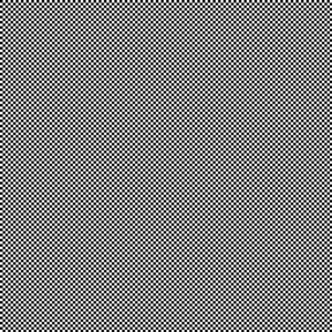
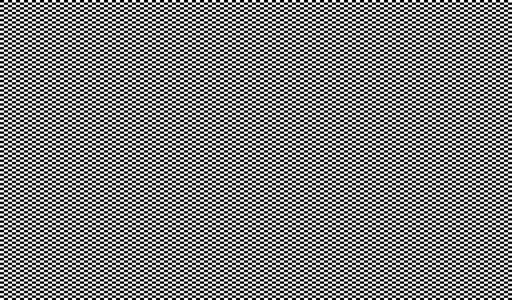
Fun Filter: Motion Blur Filter
For a fun filter, we decided to implement a subtle motion blur-like filter where each image looks at its right and left neighbors, then update its value based on theirs. It was a simple 3x3 filter whose top and bottom rows are 0s and the middle weighs the centered pixel the most.
-
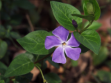
Flower
-
Checkerboard

-
Wave
Example Usage:
$ ./image -fun <input.bmp >.out.bmp